.md .pdf

repository open issue

Contents

6. Scenario Generation

If you want to calculate many sensitivities or create a scenario tree with more than 2 levels, it is better to use the Scenario Management Tool instead of the WebUser Interface. The advantage of the Scenario Management Tool is that you can create many scenarios at once.

With this tool you can create a multi level scenario tree, that has always the same number of sensitivities for each sub-scenario. You can decide how many sensitivities you want to have per sub-scenario.

In Fig. 6.1 you can see an example. Shown is a two-level-scenario-tree with 2 scenarios, 2 sensitivities for sub-scenario-one and 4 sensitivities for sub-scenario-two, it also shows how the files are named.

Fig. 6.1 Example of a 2 level scenario tree

In principle can the hotmpasDIspatch Application also calculate with different numbers of sensitivities per sub-scenario (see Scenario Mode), but mostly you want to calculate the same sensitivities over a sub-scenario.

6.1. Scenario Generation - steps for manual process

if you don’t use the the Scenario Management Tool you can create your own multi level scenario tree manually with excel files.

Note

To generate scenarios through this way, the folder structure has to look like this:

• scenario folders, named by the scenario itself

• sub-scenario files, named by the sub-scenarios; inside the scenario folder

When you want to create multi level scenario tree manually you make the following steps:

1. Copy the already existing excel files of the current sub-scenarios (e.g. when downloading the calculation in Scenario Mode, you already get the first sub-scenarios)

2. Rename the new excel files with an underline symbol.

   Tip

   The specialized structure of the sub-scenario file names helps you define the level of the scenario tree and also helps you visualize the plots for the output (See Section 6.2) .

3. Inside each excel file for each sub-scenario, the particular sensitivities have to be changed in value.

4. If you have defined and created all necessary coupled sub-scenarios and main scenarios, and you want to calculate your model, then you have to create a zip-file out of all the main scenario folders (e.g. Portfolio a,Portfolio b,… all have to be put into a zip-file)

5. Then, go to the WebUser Interface again and upload this zip-file

   Tip

   Before uploading your created zip-file, do the following steps:

   • Refresh the page, so all scenarios which were created before are deleted and no collision can cause problems

   • Enable the scenario mode

   • Then push the button Upload Power Plant Parameters and choose your zip-file

6. Before running the calculation, you can check the values which you have adapted in the WebUser Interface, if they were changed properly.

7. Push the button Run Dispatch Model for calculation

6.2. File name convention and its effect

The naming of the files describe the scenario tree levels (STL) and also how the output chart will look. The file starts with the scenario name, followed by the sub-scenario name separated by an underscore. (see Fig. 6.2).

Fig. 6.2 A general 2 level scenario tree (STL2) and the file names of the different runs

In the next chapters some examples of scenario trees are shown , and the effect of the file naming to the output charts is explained.

Note

Each data point in the charts represents a dispatch run and the input is described by an Excel file. The filename of the Excel file follows a naming convention that is specified in the heading and described in the tables

6.2.1. STL1 (a_b.xlsx)

Fig. 6.3 Example of an one level scenario tree

Table 6.1 Naming and meaning of the structure for excel files for a 1 level scenario tree

name	position in naming	Number of sensitivities and possible meaning	meaning for the plot(for system wide indicators)	meaning for the plot (for indicators by technologies)1
a	Scenario	2 technology portfolio (Portfolio a, Portfolio b)	columns2	rows2
b	Sub Scenario 1	2 \(CO_2\) Prices (Sub Scenario/1 ;Sub Scenario/2 )	x-axis and color of the data point	columns2

Fig. 6.4 Plot example of a one level scenario tree (Fig. 6.3) for a system indicator

Fig. 6.5 Plot example of a one level scenario tree (Fig. 6.3) for an indicator by technologies

6.2.2. STL2(a_b_c.xlsx)

Fig. 6.6 Example of a two level scenario tree

Table 6.2 Naming and meaning of the structure for excel files for a 2 level scenario tree

name	position in naming	Number of sensitivities and possible meaning	meaning for the plot(for system wide indicators)	meaning for the plot (for indicators by technologies)1
a	Scenario	2 technology portfolio (Portfolio a, Portfolio b)	columns2	rows2
b	Sub Scenario 1	2 \(CO_2\) Prices (Sub Scenario 1/1 ;Sub Scenario 1/2 )	rows2	columns2
c	Sub Scenario 2	2 Energy Carrier Prices (Sub Scenario 2/1 ;Sub Scenario 2/2 )	x-axis and color of the data point	shape of the data point

Fig. 6.7 Plot example of a two level scenario tree (Fig. 6.6) for a system indicator

Fig. 6.8 Plot example of a two level scenario tree (Fig. 6.6) for an indicator by technologies

6.2.3. STL3(a_b_c_d.xlsx)

Fig. 6.9 Example of three level scenario tree (For the sake of a better overview, not all edges and nodes of the graph are displayed.)

Table 6.3 Naming and meaning of the structure for excel files for a 3 level scenario tree

name	position in naming	Number of sensitivities and possible meaning	meaning for the plot(for system wide indicators)	meaning for the plot (for indicators by technologies)1
a	Scenario	2 technology portfolio (Portfolio a, Portfolio b)	rows2	rows2
b	Sub Scenario 1	2 \(CO_2\) Prices (Sub Scenario 1/1 ;Sub Scenario 1/2 )	columns2	columns2
c	Sub Scenario 2	2 Energy Carrier Prices (Sub Scenario 2/1 ;Sub Scenario 2/2 )	x-axis and color of the data point	color of the data point
d	Sub Scenario 3	2 Interest Rates (Sub Scenario 3/1 ;Sub Scenario 3/2 )	shape of the data point	shape of the data point

Fig. 6.10 Plot example of a three level scenario tree (Fig. 6.9) for a system indicator

Fig. 6.11 Plot example of a three level scenario tree (Fig. 6.9)for an indicator by technologies

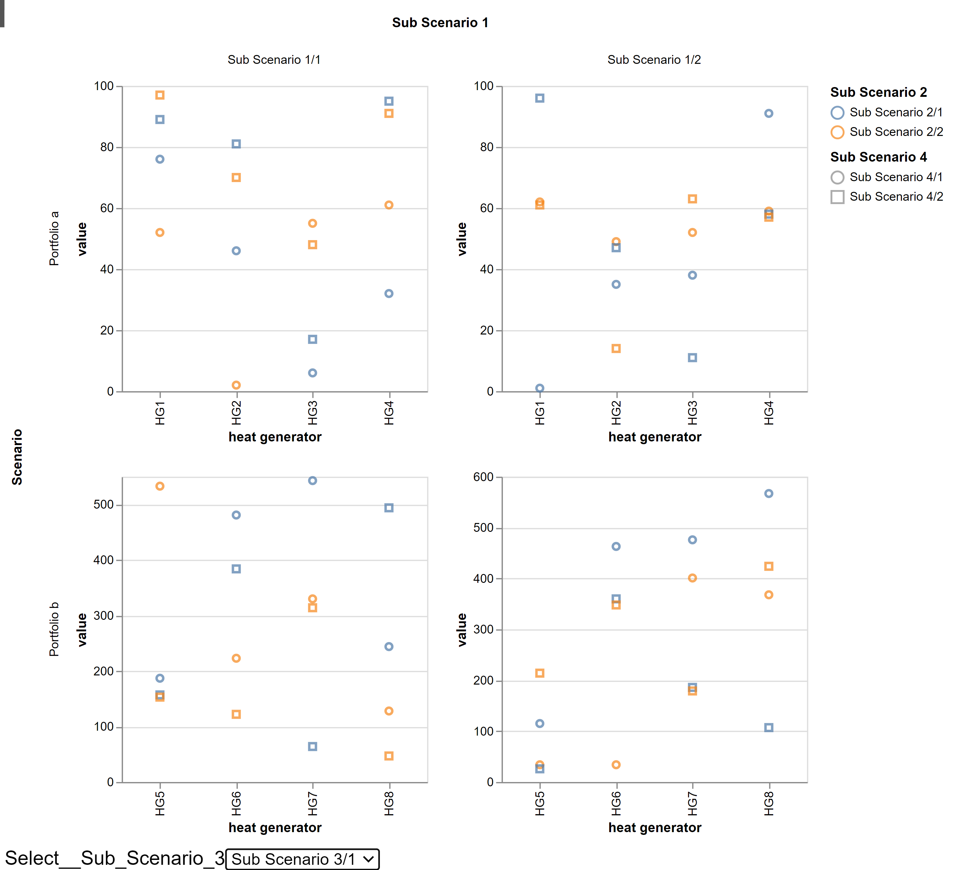
6.2.4. STL4 (a_b_c_d_e.xlsx)

Fig. 6.12 Example of four level scenario tree (For the sake of a better overview, not all edges and nodes of the graph are displayed.)

Table 6.4 Naming and meaning of the structure for excel files for a 4 level scenario tree

name	position in naming	Number of sensitivities and possible meaning	meaning for the plot(for system wide indicators)	meaning for the plot (for indicators by technologies)1
a	Scenario	2 technology portfolio (Portfolio a, Portfolio b)	rows2	rows2
b	Sub Scenario 1	2 heat demands (Sub Scenario 1/1 ;Sub Scenario 1/2 )	columns2	columns2
c	Sub Scenario 2	2 years (Sub Scenario 2/1 ;Sub Scenario 2/2 )	x-axis	color of the data point
d	Sub Scenario 3	2 Interest Rates (Sub Scenario 3/1 ;Sub Scenario 3/2 )	color of the data point	drop down menu
e	Sub Scenario 4	2 \(CO_2\) certificate prices (Sub Scenario 4/1 ;Sub Scenario 4/2)	shape of the data point	shape of the data point

Fig. 6.13 Plot example of a four level scenario tree (Fig. 6.12) for a system indicator

Fig. 6.14 Plot example of a four level scenario tree (Fig. 6.12) for an indicators by technologies

As you can see in Fig. 6.14 , there are duplicate data points that are indistinguishable. To make the data points distinctive, Sub Scenario 3 is added as a drop-down menu from a 4-level scenario tree upwards. This allows all data points to be distinctive. The illustration in Fig. 6.15 shows this approach.

Fig. 6.15 Plot Example of a four level scenario tree (Fig. 6.12) for Indicators by technologies with a drop-down menu

6.2.5. STL5 (a_b_c_d_e_f.xlsx)

Fig. 6.16 Example of five level scenario tree (For the sake of a better overview, not all edges and nodes of the graph are displayed.)

Table 6.5 Naming and meaning of the structure for excel files for a 5 level scenario tree

name	position in naming	Number of sensitivities and possible meaning	meaning for the plot(for system wide indicators)	meaning for the plot (for indicators by technologies)1
a	Scenario	2 technology portfolio (Portfolio a, Portfolio b)	rows2	rows2
b	Sub Scenario 1	2 heat demands (Sub Scenario 1/1 ;Sub Scenario 1/2 )	columns2	columns2
c	Sub Scenario 2	2 years (Sub Scenario 2/1 ;Sub Scenario 2/2 )	x-axis	color of the data point
d	Sub Scenario 3	2 Interest Rates (Sub Scenario 3/1 ;Sub Scenario 3/2 )drop down menu	drop down menu	drop down menu
e	Sub Scenario 4	2 \(CO_2\) certificate prices (Sub Scenario 4/1 ;Sub Scenario 4/2)	color of the data point	shape of the data point
f	Sub Scenario 5	2 Energy Carrier Prices (Sub Scenario 5/1 ;Sub Scenario 5/2)	shape of the data point	color or shape 3

Fig. 6.17 Plot example of a five level scenario tree (Fig. 6.16) for a system indicator

As you can see in Fig. 6.17 , there are duplicate data points that are indistinguishable. To make the data points distinctive, Sub Scenario 3 is added as a drop-down menu from a 5-level scenario tree upwards. This allows all data points to be distinctive. The illustration in Fig. 6.18 shows this approach.

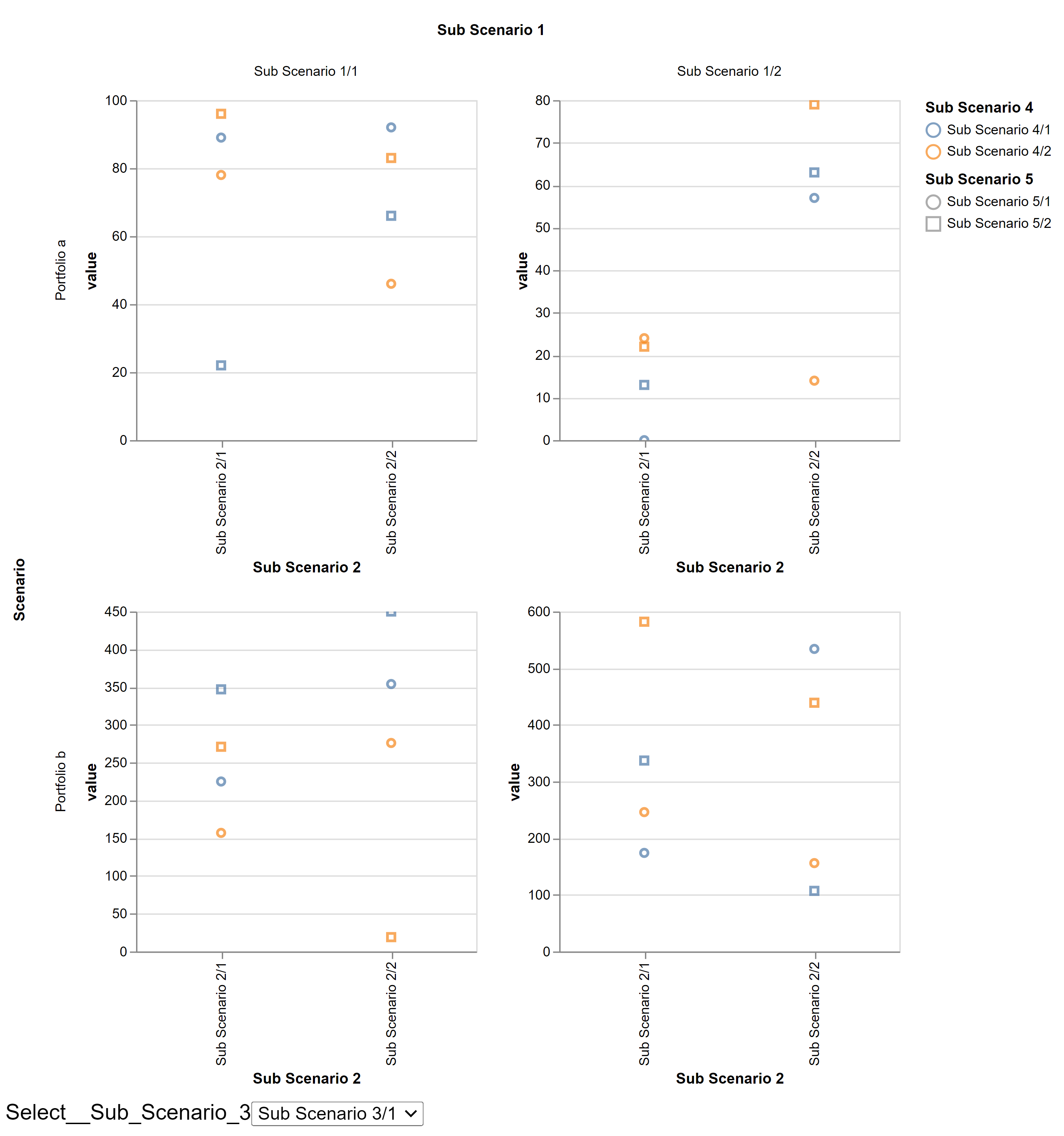
Fig. 6.18 Plot Example of a five level scenario tree (Fig. 6.16) for a system indicator with a drop-down menu

The illustration in Fig. 6.19 shows that from a 5-level scenario tree onwards, even the addition of a drop-down menu does not make it possible to visually create a clear allocation of the data points. Of course, one can now create a drop-down menu for each additional sub-scenario, which would solve the problem with the ability to distinguish the data points, but the chart itself would not become clearer, nor would it be possible to publish analogue graphics (for papers, for example).

Fig. 6.19 Plot example of a five level scenario tree (Fig. 6.16) for an indicators by technologies

---

Warning

It is not advisable to calculate scenario trees deeper than 5 levels (Fig. 6.16), as the results of the sensitivities are no longer straightforward to visualise and therefore can no longer be easily analysed and interpreted.

6.3. Scenario Management Tool

The main advantage of using the Scenario Management Tool is to only use two kind of files, whereas you separate which values stay constant and which parameters will change, this safes time and effort.

Two files are being used for generating scenarios (Fig. 6.20):

• default_input_dispatch.xlsx

• scenarios.xlsx

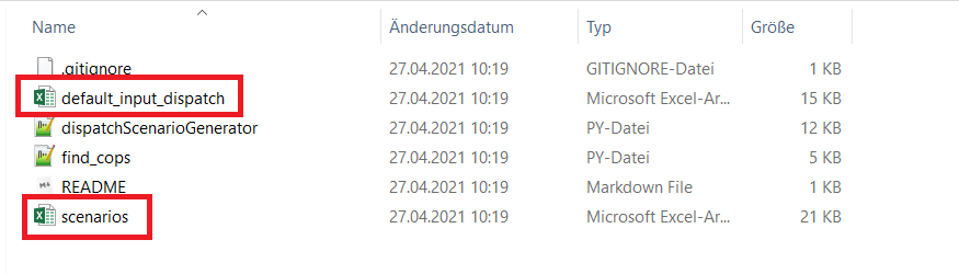
Fig. 6.20 Necessary excel files for scenario generation.

6.3.1. default_input_dispatch.xlsx

All values/parameters will be defined here which won’t change for this run. There are predefined worksheets, which are shown in Fig. 6.21.

Fig. 6.21 Possible options for setting default values.

Each worksheet has empty gaps to be filled up if necessary, as shown in Fig. 2.3.

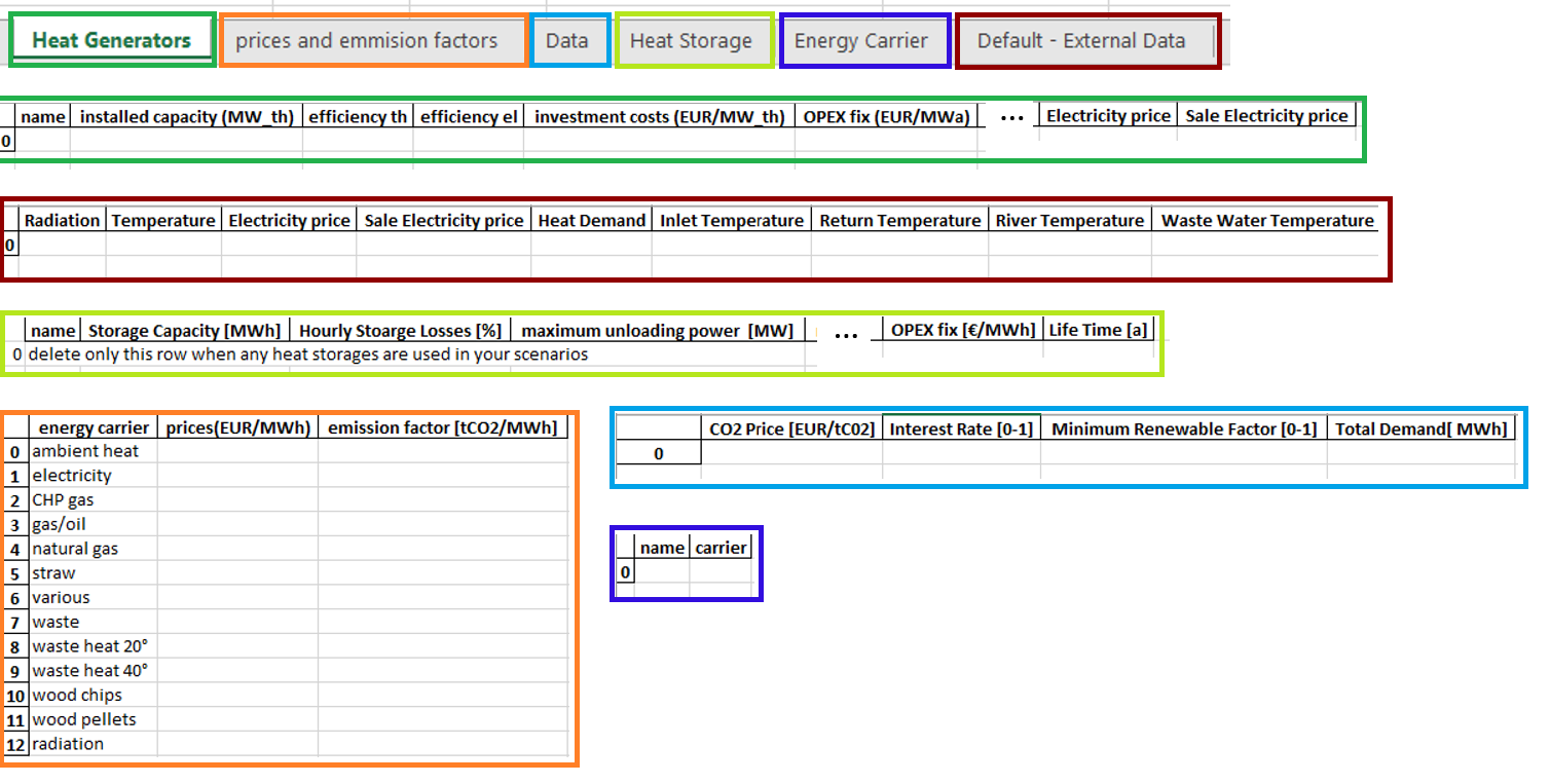
Fig. 6.22 Predefined values to set.

6.3.2. scenarios.xlsx

• All values/parameters, which will be changed, will be added in the worksheets in Fig. 6.23.

Fig. 6.23 Predefined worksheets to fill in.

Warning

Delete all the values/parameters you don’t want to vary and define individual names for each scenario/sub-scenario and coupled ones. If you don’t want to make any specifications at a worksheet, however you have to put in the names of your portfolios and the number in the first column, like in Fig. 6.24. The other columns you can left blank.

You can choose the number of portfolios which you want to create and the type of heat generators. In Fig. 6.24 there are different portfolios with its heat generators filled in each column (here A,B,C etc.). The different shades of the pink boxes just emphasize the different portfolios, but in general you are free to create as many as needed.

Warning

All the different worksheets in excel can be almost chosen freely, depending on the different sensitivities you want to calculate. However, the names have to start the same way as predefined in the default_input_dispatch.xlsx:

• All worksheets here have to start with the specific sensitivity category (e.g.: for different electricity prices you need the Profile worksheet)

• Then, add a minus afterwards and a corresponding name for your sensitivity case (e.g.: Profile - Electricity Prices or Data - interest rate) .

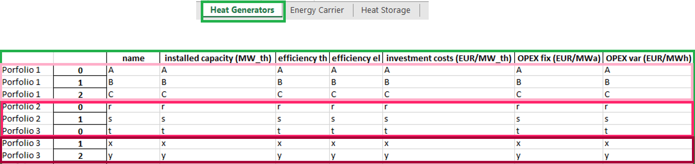
Fig. 6.24 Heat generators and portfolios definition.

Tip

If you want to use the same technologies for all portfolios (but e.g.: with different capacities), to get a better overview of the output plots, you should name the heating technologies equally for each portfolio, but with a space character afterwards the name, so that it will be treated as different values while runing the model, but to be plotted as the same technology to be comparable.

In Fig. 6.25 you can define the specified name and energy carrier for each portfolio.

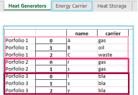
Fig. 6.25 Energy carrier definition.

Defining different heat storages is possible like in Fig. 6.26.

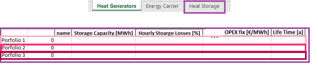
Fig. 6.26 Heat storage definition.

You can define a sensitivity for profile, which will be adapted like in Fig. 6.27.

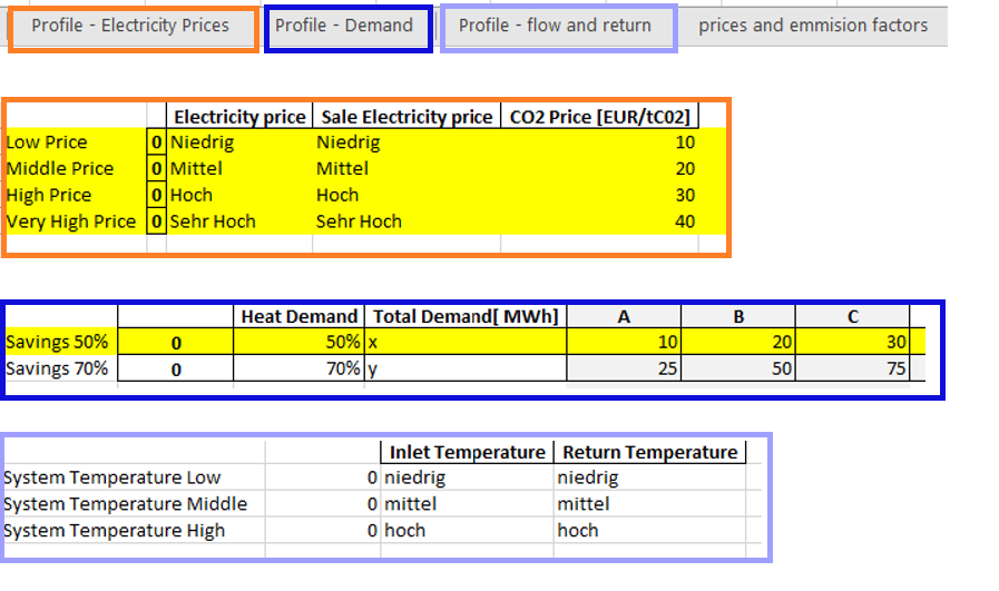
Fig. 6.27 Examples of profile sensitivities.

For defining different sensitivities (e.g.: different gas prices, held in light and dark green in the figure), you have to adapt the following worksheet in Fig. 6.28. It depends on the number of sensitivities how many “green boxes” you have create in that worksheet.

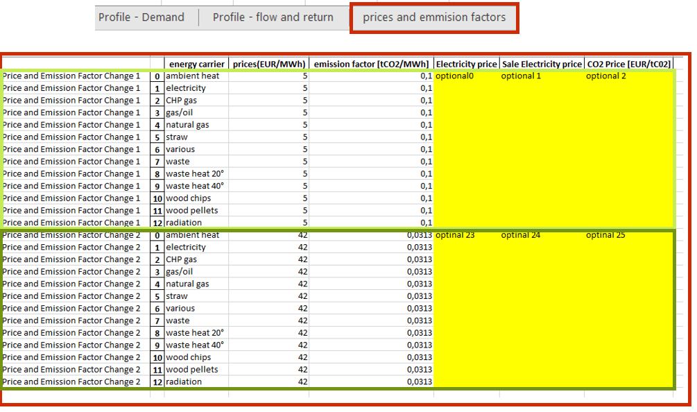
Fig. 6.28 Sensitivity setting via price definition.

Additionally, you can define an interest rate, like in Fig. 6.29.

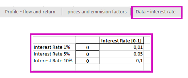
Fig. 6.29 Interest rate definition.

Tip

If you want coupled sensitivities, you have to add the one you want to couple to the one which is defined in a worksheet. For instance, if you want to combine the effect of electricity prices with \(CO_2\) prices, then you add a column for \(CO_2\) prices in the worksheet where you defined the electricity price sensitivity.

If everything is defined correctly, then dispatchScenarioGenerator.py has to be executed, see Fig. 6.30.

Warning

Inside the python file dispatchScenarioGenerator.py: Change the path of your input path for your dat-files, which should be the one where you cloned the repo in the beginning.

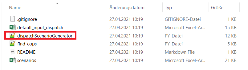
Fig. 6.30 Execute the python file

• After the code run, it creates an output folder, where you have as many folders as generated scenarios. Inside them, you find all your excel files with the sub-scenarios and varying sensitivities.

• To calculate the model, a zip-file has to be created out of all the portfolio folders. Then you can upload it, like described in this chapter before, with the button Upload Power Plant Parameters and check again, if the values you changed, fit.

• The last step is the calculation via the button Run Dispatch Model

---

1(1,2,3,4,5)

(The x-axis is always reserved for the heat generators, therefore the scenarios and sub-scenarios must be adjusted accordingly)

2(1,2,3,4,5,6,7,8,9,10,11,12,13,14,15,16,17,18,19)

(for each row and column a figure is created)

3

(random selection)

5. Investment Mode 7. Example Projects